Principle Component Analysis (PCA)
Dimensionality reduction
About
Dimensionality reduction is a technique used in unsupervised learning that allows you to observe the “most important” dimensions of a set of data
.
More specifically we want to transform a set of
data points that each have
features to a set of
data points that each have
features where
. The goal is to reduce the dimension of data points while preserving as much information from the original data as possible.
This can be helpful for many reasons:
Computational efficiency
Improved learning
Some algorithms’ assumptions are better satisfied in low dimensions. Also, dimensionality reduction can act as a regularizer
Pre-training
We can learn the “good features” that should be used for supervised learning from very large amounts of unsupervised data.
Visualization
It is much easier to plot low dimensional data.
Objective
Lets assume that each of the
data points
where
is a very high dimensional space. We want to find a compressed representation of
using some function
such that
where
. We also want to maintain that
retains the “information” in
.
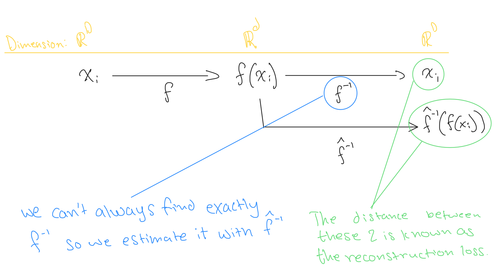
Consider the estimated inverse of
denoted
, that attempts reconstructs
from
. Our goal is to make functions
such that the following distance is minimized:
This is known as the reconstruction error.
Principle Component Analysis
Principle component analysis is one way can do this dimensionality reduction and minimize the reconstruction loss.
Suppose we are given
data points
and
is the target dimensionality we want to reduce to. In PCA, we find a linear transformation
that maps all
from
. When choosing
we want to preserve the structure of data.
Specifically, we find an
orthogonal projection
using a matrix of orthonormal row vectors
. So our reduction function
is
. Since the rows of
are orthonormal, they make an orthogonal basis for
.
We can therefore define the estimated reconstruction (inverse) function
directly using
. So we have
. Note that this is an “estimated inverse” function since
doesn’t always give back exactly
. Instead, it gives back an estimated “reconstruction” of
.
💡
Note for PCA to work correctly, we assume that the mean of our data is 0 and it has unit variance. We can simply subtract the mean and divide by the standard deviation across each dimension of
to achieve this. An intuition for why we are doing this is that we want to make sure that no dimension is more “important” than another.
PCA as Minimizing the Reconstruction Loss
Recall that the reconstruction is given by
where
and is composed of orthonormal row vectors
and
. Since
is composed of orthonormal vectors we know that
(identity matrix of dimension
).
The reconstruction error for the
th point is then:
We can rewrite
as
and rewrite the above as:
Until now we considered
. But what if
Well, then we would for some matrix
:
. Since
is also composed of orthonormal vectors,
would now be an orthogonal matrix and
(identity matrix of dimension
). Therefore we know:
for some sequence of orthonormal vectors
.
So we have
. Plugging this back in for the reconstruction error for
we get:
Since we are trying to minimize this error, we can formally write this as an average over all data points as:
Using some algebraic manipulation, we can simplify this optimization to:
This is equivalent to maximizing over the first
vectors:
So how do we solve this? Recall that
and
results in a vector in
To maximize
we know
must be in the direction of
. This is because for an arbitrary vector
, the dot product of
is maximized when
by properties of the dot product. Therefore, we want
to be a vector such that
for some scalar
.
In order for
to hold,
must be an eigenvector of
. Therefore, we will get
where
is an
eigenvalue
of
and
is an
eigenvector
of
.
Now, which eigenvector/eigenvalue pair do we choose?
Well, since
, then
. Since we are maximizing over the space
where
, we know that
.
Now the eigenvector/eigenvalue we choose is trivial. We simply choose the
eigenvalues
and its corresponding eigenvectors that are the greatest! Note, the largest eigenvalues of a matrix are known as the
principal
eigenvalues.
This means if we take
as the
eigenvectors corresponding to the
largest eigenvalues of
, we can construct a matrix
and use
to project
using the transformation
.
Computing the eigenvalue
Now one question remains, how do we compute the eigenvalues/eigenvectors from
?
Well we can simply just compute the eigen-decomposition. (recall the procedure of solving
, and solving the characteristic equation).
While this works, it is a bit slow. Computing
for the covariance matrix takes
time, followed by the
time to compute the eigen-decomposition.
A faster method is to use the singular value decomposition (SVD) of
. This is given by:
I won’t get into the details of this here but just know that it runs in faster
time.
Algorithm
Formally, our algorithm to reduce
points of
dimensional data to
points of
dimensional data (
is:
Let
be our dataset
Normalize
such that it has mean 0 and standard deviation 1
Compute matrix
Conventionally
is done over
as this comes from the
maximizing variance formulation of PCA. However, both are equivalent as this just results in a different scaling of the eigenvectors.
Find the
principle eigenvectors (eigenvectors corresponding to largest eigenvalues), denoted
of
using either eigen-decomposition or SVD.
Create a matrix using the eigenvectors
.
Create the dimensionality-reduced dataset by
-
Sources


varchi [at] seas [dot] upenn [dot] edu.