Variational Autoencoders (VAEs)
Variational autoencoders for generation
About
Variational Autoencoders (VAEs) are models that can be used to
generate
new images similar to ones seen in a training dataset.
While VAEs themselves aren’t directly used in modern generative models, they form a basis for many of them including diffusion models.
Latent Variables
Since latent variables are at the heart of VAEs, it is important to define what they actually are.
If you have heard about latent variables before, you might have heard them described as hidden variables that determine the observed variables. I had a hard time wrapping my head around this so I will give a few examples:
Say you have a bunch of students who took an exam for the course MATH 101. Trivially, the observed variables are the exam scores. However, a latent variable would be the amount of MATH 101 that was actually learned by each student.
- Plato’s Allegory of the Cave
. Lets say that you were born and raised inside a cave. You have never left this cave your entire life. Every day at dusk, there are people who walk by the outside of the cave. Due to the sun, you see shadows of these people cast into the cave. You never know what the people who are casting the shadows look like, instead you can only
observe
the shadows. Here the latent variables are the humans on the outside of the cave casting/controlling the shadows.
Le
t’s say you have 2 variables
. These 2 variables are used to produce 5 dimensional vectors that are functions of the 2 variables.
For example:
. We only
observe
the 5 dimensional vectors for different values of
and
. You can think of
and
as controlling the changes in the 5 dimensional vectors. Therefore,
and
are the latent variables.
High Level Overview
In VAEs, we essentially train and “organize” a latent space (vector space of latent variables).
We do this by using a neural network to take a high dimensional input vector
to a lower dimensional vector
in the latent space. We then use another neural network to take
back into a higher dimensional vector
which is the same dimension as
. Our network is trained to both “organize” (I will expand on what “organize” means later) the latent space and reduce the difference between
and
.
To generate new data, we simply take a random sample from the latent space and use the second neural network to produce a vector in the input space.
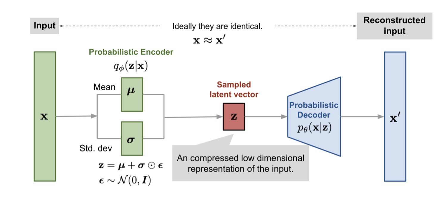
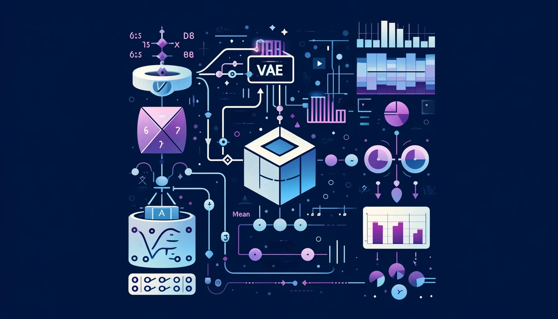
Overview of VAE architecture. Source: Lilian Weng
https://lilianweng.github.io/posts/2018-08-12-vae/Autoencoders
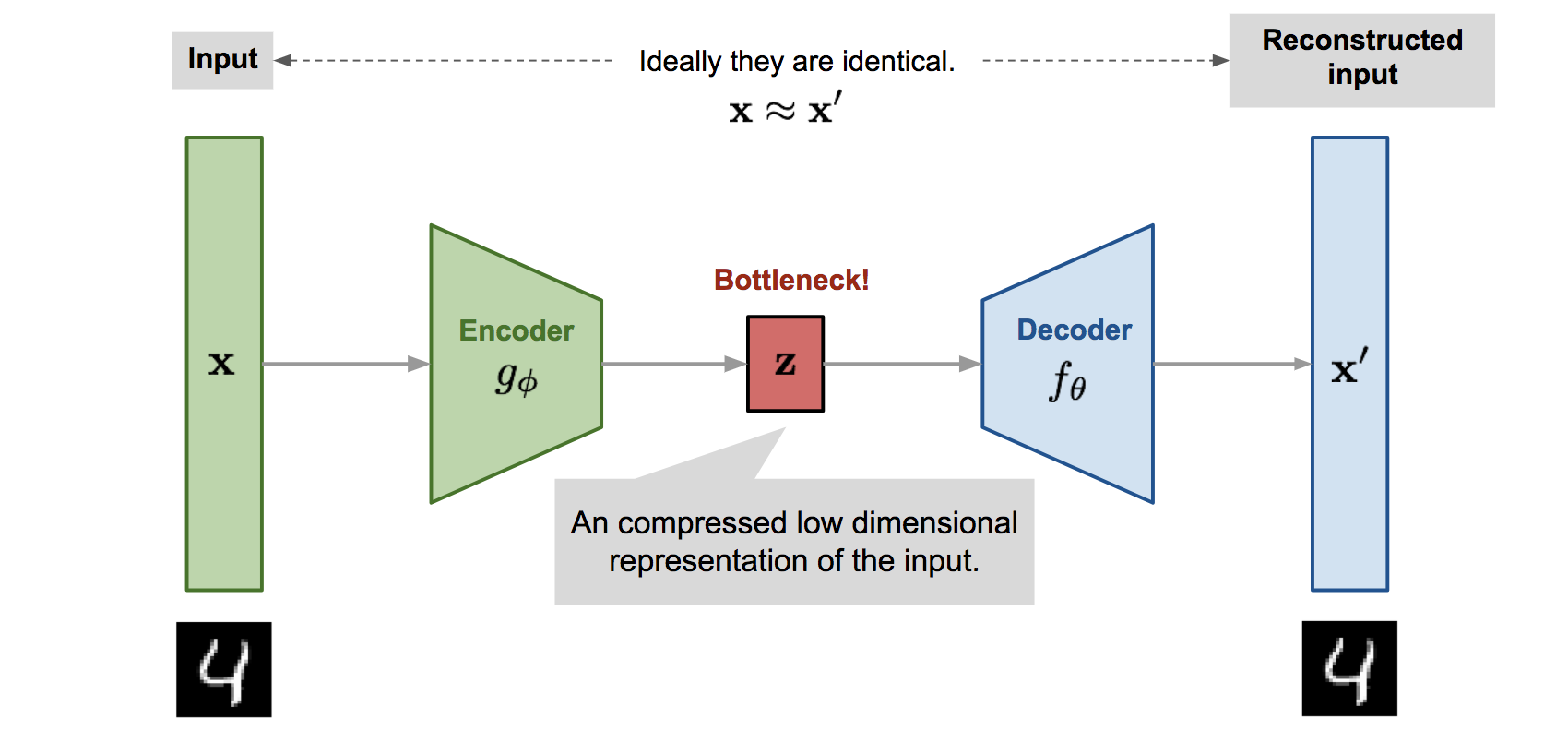
Before we talk about VAEs, we should talk about autoencoders.
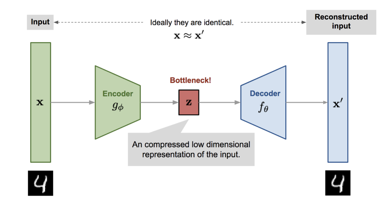
Illustration of an autoencoder. Source: Lilian Weng
https://lilianweng.github.io/posts/2018-08-12-vae/Autoencoders are models that try to learn low dimensional representations of input vectors. The low dimensional representations should contain the “most important” features of the input vector. This allows you to (approximately) reconstruct the original input vector from the low dimensional vector.
Observe how this is very similar to
PCA. Recall that PCA uses a linear transformation (matrix) to go from a high dimensional vector to a low dimensional vector and then a second linear transformation (matrix) to go from the low dimensional vector to a high dimensional vector. PCA then tries to minimize the difference (reconstruction loss) between the 2 high dimensional vectors. Autoencoders do the same, but instead of going from different dimensions using linear transformations, it uses neural networks. One neural network (encoder) decreases the dimension and another neural network (decoder) increases it. This is why a lot of people refer to autoencoders as a kind of non-linear PCA.
In autoencoders, the space of low dimensional vectors can be thought of as the space of latent variables i.e. the latent space.
Autoencoders for Generation
You may now be thinking that to generate new content, we can simply take a random sample of the latent space and use the decoder neural network to get a vector that is the same dimension as our input vectors.
However, this won’t work because the latent space isn’t “organized”. Meaning a random sample is likely to produce gibberish.
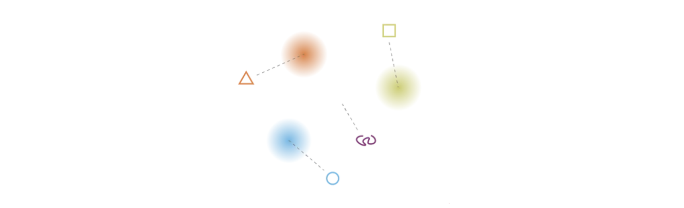
Latent space model. Source:
https://towardsdatascience.com/understanding-variational-autoencoders-vaes-f70510919f73The above image tries to model a latent space. The gradient colors represent regions in the latent space that, if sampled and passed through the decoder neural network, will produce some meaningful reconstruction (like the triangle, square, and circle). However, notice how taking a random sample of this space is likely not going to fall in one of these gradients. Decoding a sample from the white space is going to produce gibberish, like the purple squiggly line.
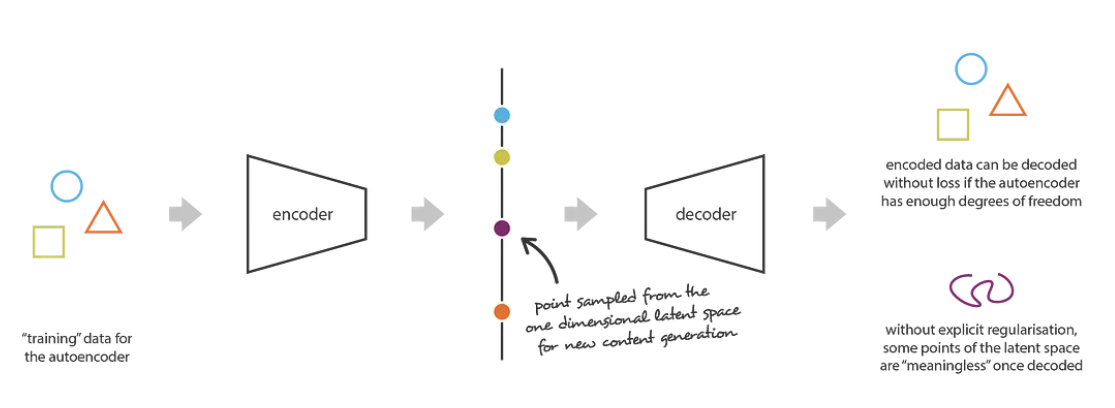
Irregular latent space prevents use from using autoencoder for new content generation. Source:
https://towardsdatascience.com/understanding-variational-autoencoders-vaes-f70510919f73We need some way to “organize” this space so that the majority of samples fall in these gradients.
VAEs
Definition
A variational autoencoder can be described as a model that not only tries to learn a good latent space, but also “organize” it such a way that random samples of the space can produce meaningful results.
💡
VAEs achieve this by trying to learn the probability distribution of the latent space.
VAEs are similar to autoencoders in that they use
probabilistic
encoders/decoders instead of normal encoders/decoders. This means that instead of using neural networks to get a vector in the latent space given a vector in the input space (and vice-versa), it uses neural networks to get a probability distribution of the latent space given an vector in the input space (and vice-versa).
Math
Objective
For all observed data
, we assume they are i.i.d. and come from some underlying probability distribution
. We then try to learn a model that generates a probability distribution
, for model parameters
, such that the likelihood
is maximized for all observed data points. This approach is called
likelihood maximization.
We can imagine the latent variables
of the observed data as modeled by a joint probability distribution
. By chain rule of probability, we have
. We also have
by marginalization. Directly computing
and trying to maximize it is difficult because you would have to either have access to the ground truth distribution of the latent encoder,
, or integrate all latent variables
out (intractable for high dimensional
).
Instead we try to approximate
.
Let us first formally define our objective. As with many other probabilistic models, we try to maximize the log-likelihood of the observed data.
Since we don’t have access to
, we try to estimate it with a variational distribution
for parameters
. More specifically,
The last step follows from
Jensen’s Inequality. The last term,
, is formally known as the evidence based lower bound (ELBO). Since it is a lower bound, maximizing this will also maximize the log-likelihood:
.
ELBO can be simplified even further (and makes the objective function of VAEs more apparent)
Here
is known as the
KL-divergencewhich is a measure of how close 2 probability distributions. Note that the KL-divergence is a non-symmetric measurement, but that is not too important right now.
We try to match
to
by reducing the difference (KL-divergence) between
and
. This works because
is an upper bound on
.
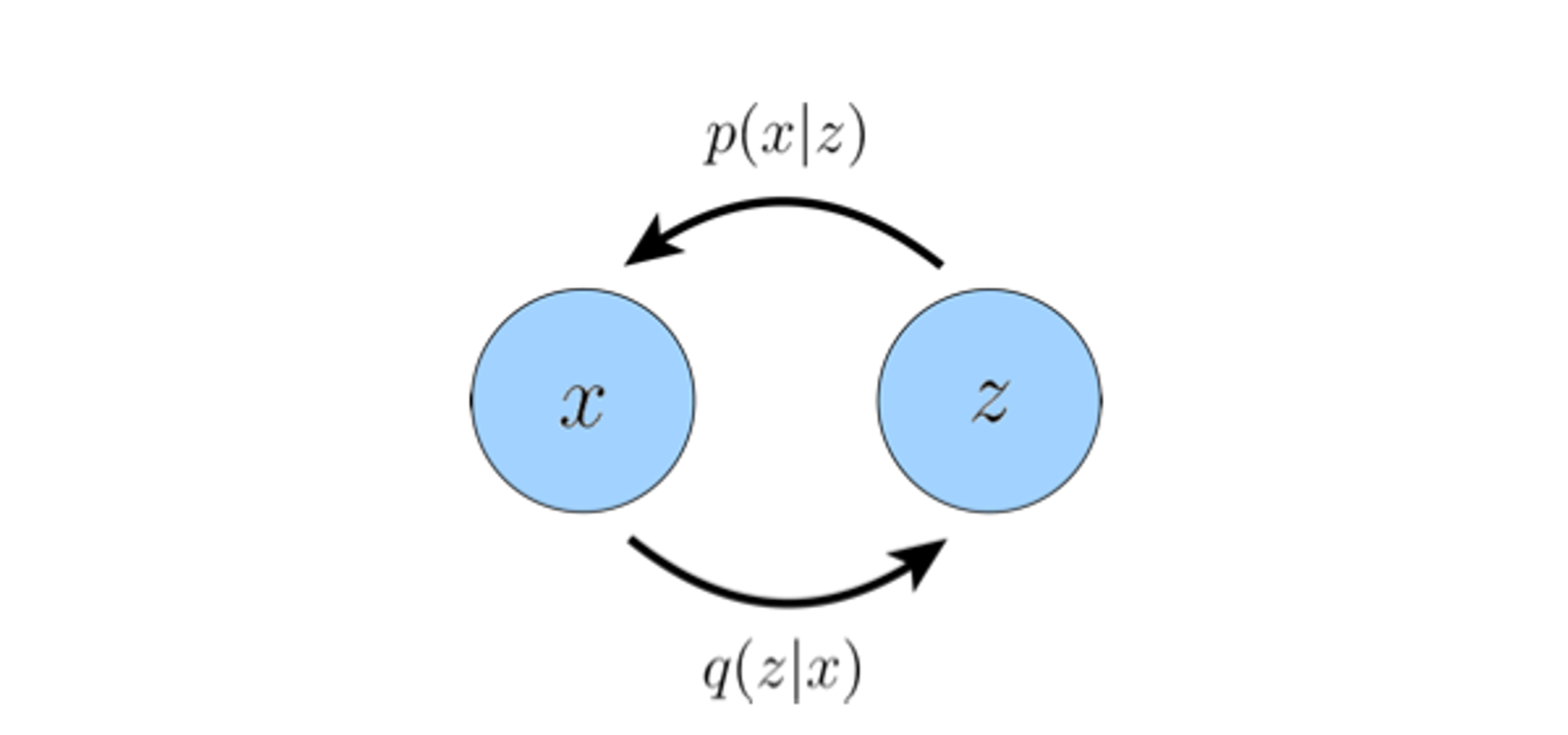
Note that
gives a probability distribution of latent variables
given an observed variable
. Therefore,
can be thought of as a
probabilistic encoder
. Similarly,
gives a probability distribution of observed variables
given a latent variable
. Therefore
can be thought of as a
probabilistic decoder
.
Once again, our objective is to maximize ELBO over parameters
where ELBO is:
Optimizing
We first look at the second term in ELBO which is KL-divergence.
In VAEs, when trying to maximize ELBO, we assume
to be the standard multivariate gaussian.
We also assume
to be some multivariate gaussian with diagonal covariance.
This means we learn models
and
, which are smaller neural networks, in order to create a mean vector and a standard deviation vector given a datapoint
.
Since we are trying to reduce the KL-divergence and bring
as close to
as possible and
is the standard normal distribution, we are essentially trying to bring the distribution of all latent variables to the standard normal distribution. This is how we “organize” the latent space.
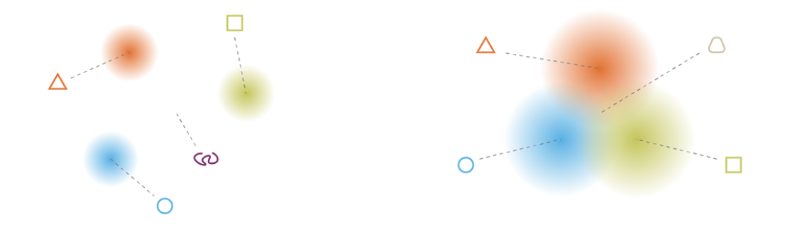
The returned distributions of VAEs have to be “organized” to obtain a latent space with good properties. Source:
https://towardsdatascience.com/understanding-variational-autoencoders-vaes-f70510919f73We now look at the first term in ELBO:
. This term tells the model to maximize the log-likelihood for seeing the input data
given latent representation
.
Since we don’t have access to all possible latent variables
, we instead estimate this expectation using a
Monte-Carlo estimate. Specifically, we do:
This means for some relatively small
, we sample
and compute
. In practice, if the dataset is large, we can use
.
There is still one small problem though. Since sampling is a non-differentiable procedure, we can’t just simply generate samples from
. This is because we want to be able to differentiate
and
during back propagation.
Instead, we employ a method called the reparameterization trick. This trick rewrites
as a deterministic function and offloads the randomness/sampling to a random variable
. Note that
doesn’t need to be differentiated because it is not learned.
Therefore instead of sampling
, we first sample
and then say
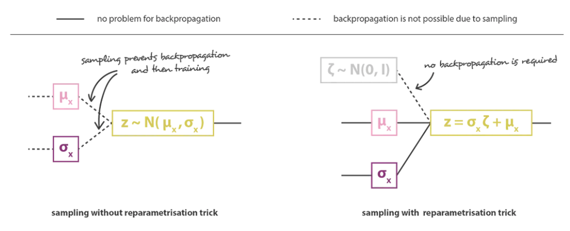
Illustration of the reparametrisation trick. Source:
https://towardsdatascience.com/understanding-variational-autoencoders-vaes-f70510919f73That’s it! We now have a well defined objective function to optimize over. Maximizing the
term of ELBO tells our model to look for latent representations that allows for the reconstruction to be as close to the initial input and the
term of ELBO tells our model to “organize” the latent space for good sampling during generation.
In practice, however, we don’t use the probabilistic decoder
to once again model the distribution and compute
. Instead, we directly compute
(reconstruction of
) from
using the probabilistic decoder neural network and try to make it as close to
as possible. That is we try to minimize
for some loss function
instead of maximizing
.
Overview of VAE architecture. Source: Lilian Weng
https://lilianweng.github.io/posts/2018-08-12-vae/Code
We use the following libraries and starter code:
Loading the data
Loss term
Recall that we are trying to maximize the ELBO which is formally:
Let’s look at the first term which is
. Recall that in practice, we don’t use the decoder neural network to model the distribution
, but instead just use it to directly compute
from
which is a reconstruction of
. Therefore, maximizing this is equivalent to minimizing the reconstruction loss between
and
. Therefore, we use the
binary cross entropy losswhich is a good loss to measure reconstruction. Note that other losses can be used, such as
MSE loss. So instead of
we do:
Now let’s look at the second term which is
. Instead of maximizing the negative of the KL-divergence, we simply just minimize it. Recall that we assume
to be the standard normal distribution
and
to be the normal distribution
. Using the formula for KL-divergence on
dimensional multivariate gaussians and simplifying based on the fact that
, we get that the KL-divergence is:
Note that the
can be omitted because it is a constant.
Putting this into code, we get the following:
Approximated ELBO loss function
Note that we chose to multiply the KL-divergence by a positive constant in order to tell the model to put more weight on organizing the latent space. This allows for slightly more meaningful generation.
VAE Model
The VAE model is essentially just a bunch of neural networks.
More specifically, for a latent space dimension
, the probabilistic encoder is a neural network that takes an input vector and produces a
dimensional mean vector (representing
) and a
dimensional standard deviation vector (representing
).
The probabilistic decoder is another neural network that takes a
dimensional vector in the latent space and outputs a vector in the input space.
For the model, we chose to use a mix of non-linearities. The most important part is that we have
non-linearities at the end of our probabilistic encoder network layers (in order to constrain the outputs between -1 and 1) and a
non-linearity at the end of the decoder layer (to allow for good inputs for the
term in the loss function).
VAE model
Training Loop
The training loop is defined as usual:
Results
The results and all the code can be found at:

Decoding
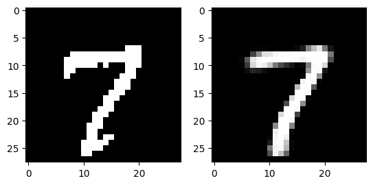
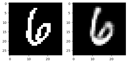
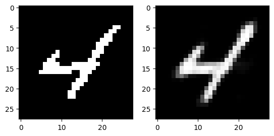
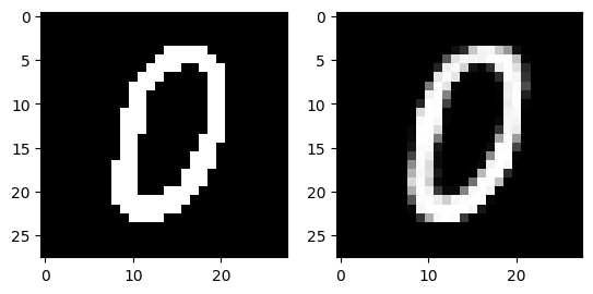
The following images are reconstructed from a single pass through the model. The image on the left of each figure is the original image from the dataset and the image on the right of each figure is the reconstruction.
Generation
The following set of images are generated by randomly sampling vectors in the latent space and decoding them using the model.
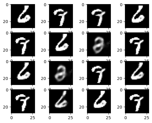
Generation of random samples from latent space.
-
Sources


varchi [at] seas [dot] upenn [dot] edu.